Welcome to part 3 of this tutorial. In this part, we will learn about representing signals in the frequency domain with Fourier analysis. If you missed part 2, check it out here. This part of the tutorial will likely be the last. I may also return to discussing related content in other series’ for example, the visualising audio series which I plan to write soon.
The Frequency Domain
In the previous sections of this tutorial, we have been discussing audio signals in the time domain. In other words, we had time along the x-axis and amplitude along the y-axis. Analysing waveforms in the time domain is very useful for understanding how the air pressure varies between instances but not very useful for telling us how a signal will sound. This is because humans hear pitch, timbre and harmonics which are all frequency based.
An alternative way to view audio signals is in the frequency domain. Rather than considering the air pressure at each moment in time, we instead consider which frequencies are present over a period of time. An important limitation of the frequency domain is that we cannot describe frequency at a single instant, only an average over a window of time.
To understand why, consider the analogy of a car driving down the road. In the time domain, we plot the position of the car against the time. If we want to understand the speeds involved, however, we cannot measure speed at an instant. We must instead compare positions across smaller time intervals. Frequency behaves in the same way. It describes how a signal changes over time, not its value at a single moment.
Fourier Analysis
In order to transform the audio signal to the frequency domain, we can use Fourier analysis. This method, named after French mathematician Joseph Fourier involves transforming a raw audio signal into its single frequency components. This works due to a key property of signals: any periodic signal can be represented as a sum of sine waves with different frequencies, amplitudes, and phases. This is not just relating to simple tones but any waveform! For example, a square wave consists of a fundamental sine wave plus its odd harmonics with amplitudes proportional to 1/n. An example of breaking a simple waveform down into its components can be seen below.
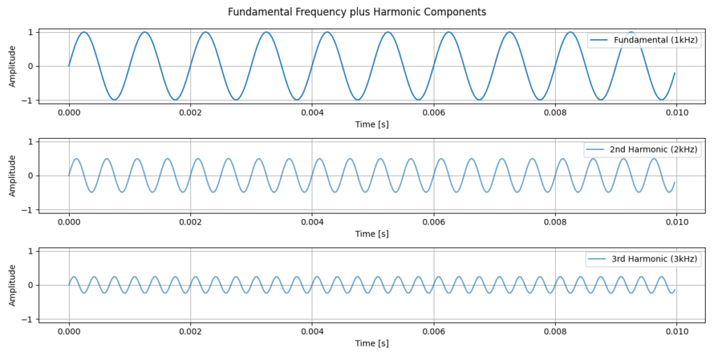
In the plot above, we can see a fundamental frequency plus two of its harmonics, where each harmonic has an exponentially lower amplitude. Looking at the signals, it’s not immediately obvious how they will look once combined. We can see a combined example below.
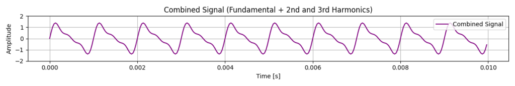
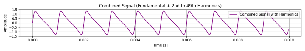
In the combined signals above, we can see that once we combine each of the harmonics, with the fundamental frequency, we are starting to get a negative ramp saw wave. The first plot contains only 3 sine waves and is already quite close to a saw wave already. Once we get to the 49th Harmonic, the wave is significantly smoother and the attack is much faster. This example perfectly demonstrates why it is important to use the frequency domain for some signals. Using the time domain, anyone familiar with sound synthesis will be able to imagine how this sounds. However, most people won’t know what frequencies are contained within the signal. Using Fast Fourier Transform (FFT), we can efficiently compute this decomposition and transform a time-domain into its frequency-domain representation.
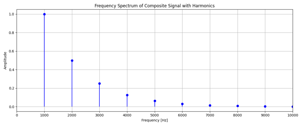
The y-axis here is showing the amplitude or in other words, the magnitude of each frequency that is present within the signal. We can see that the magnitudes of each frequency quickly tends towards zero. This is why the wave with only 3 harmonics already looked very close to its final form. It is important to also notice that when analysing these waves, it is useful to interpret both the time and frequency domain. It is common to do this in many practical applications, since each of the graphs provides us with different information.
A key limitation of performing a Fourier transform across the entire length of an audio signal is the inability to capture changes over time. For example, consider a signal that changes frequency halfway through. A single FFT of the full signal may suggest that both frequencies were present simultaneously, when in reality they occurred sequentially. This illustrates a fundamental trade-off in signal processing. We cannot have perfect resolution in both time and frequency simultaneously. Increasing the frequency resolution requires analysing longer time windows, while capturing rapid changes in time requires shorter windows.
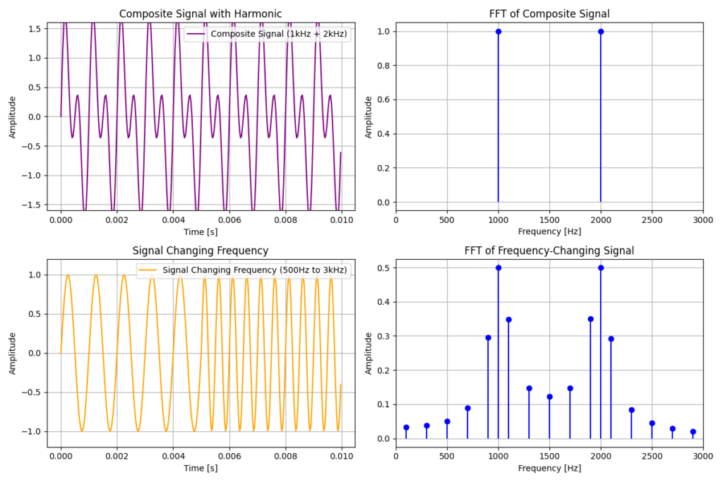
Something to note in the above figure is that the FFT of the signal that changes frequency half way contains more frequencies than just the 2 frequencies which are truly in the signal. This happens due to FFT fitting to other frequencies on the boundaries between the waves. To overcome issues with changing waveforms, we can instead use a Short-Time Fourier Transform.
Short-Time Analysis and Spectrograms
In many real world applications, audio signals are non-stationary, meaning that they change over time. Musical notes evolve, speech changes from phoneme to phoneme and environmental sounds appear and fade away. To analyse how frequencies change over time, we need to look at short sections of the signal where the frequencies can be considered approximately stable.
To do this, we use windowing. Windowing involves multiplying the signal by a window function such as Hann, Hamming or Blackman window. This isolates a short segment of the audio while smoothly reducing the influence of samples at the boundaries of the window. We then apply a Short-Time Fourier Transform (STFT), which takes a windowed chunk of audio, performs FFT, shifts the window forward in time and repeats the process.
Below we see an example of this process applied to an audio signal with many changing waveforms.
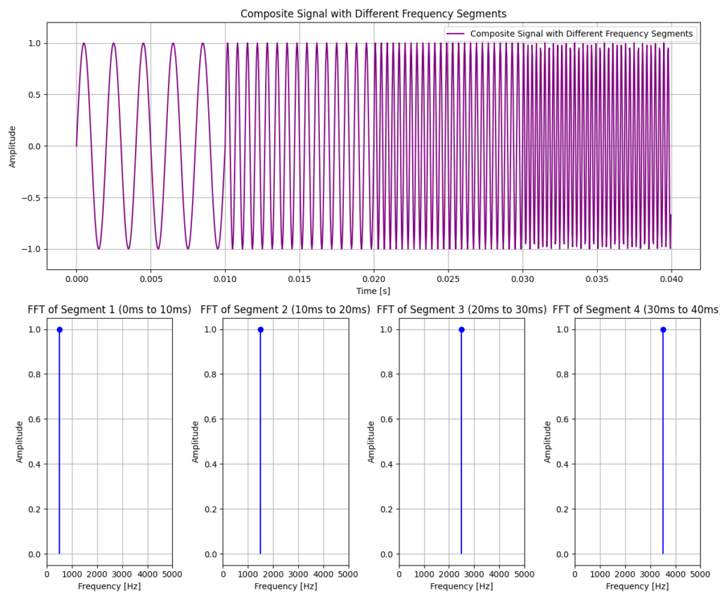
As the window moves through the signal, a new Fourier transform is computed at each position. This prevents parts of the signal outside the window from influencing the frequency analysis at that time.
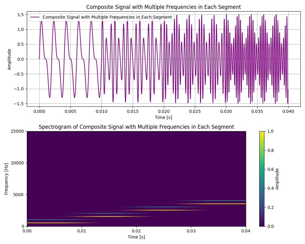
While it can be useful to view the frequency content of individual windows, it is often more informative to see how the frequency evolves over time across many windows. For example, when analysing audio clips with tens of thousands of windows.
To do this, we use a spectrogram to view a time-frequency representation of a signal. A spectrogram is constructed by computing the STFT for each of the windows and arranging the resulting spectra along a time axis. Below is a spectrogram of the previous signal.
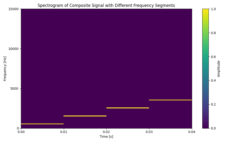
We can see that each of the frequencies are represented by a horizontal line, with brighter colours indicating higher magnitudes. This representation allows us to clearly see when frequencies appear, disappear or change over time. I will end this tutorial with a more complex example containing multiple simultaneous frequencies.
Thank you for following along with this short tutorial series. I learned a lot while writing this series and I hope it has helped build an intuitive understanding of how audio signals are represented and analysed on a computer!
Until next time,
Emily