In the first part of this tutorial, I covered the basics of audio conceptually. You can find this here. In this part of the guide, I will shift our focus to the key part of this tutorial, computer audio. I begin with an introduction of sampling and representing sound, before exploring some operations and analysis techniques.
From Sound Waves to Digital Signals
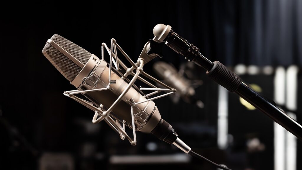
Audio Recording Equipment
To begin part 2 of the tutorial, I think it makes most sense to discuss how audio can actually be input into the computer. The most obvious way here is to use a microphone. A microphone is a physical device which contains a small membrane. As the soundwaves hit the membrane, they cause it to vibrate with the same waveform as the soundwaves in the air. For one type of microphone, the dynamic microphone, the membrane is attached to a small wire coil, which surrounds a small magnet. As the coil moves around the magnet, from the vibration, current is induced within the coil circuit.
The current within the circuit gives us an electrical representation of the audio signal. The last step is to process the electrical signals into a digital signal by using an ADC (Analog to Digital Converter). This is a specialised piece of equipment, which converts continuous analogue signals into discrete digital ones.
Sampling Sounds
A key aspect of working with digital representations of sound waves is representing signals in the time domain. Put most simply, this means representing the soundwave as time passes. In part one, I discussed that soundwaves are physically made up of air particles which cause changes in air pressure as they travel. The representation of the soundwave is just the amount of air pressure deviation at the microphone diaphragm over time. This can theoretically be considered as a mathematical function, where the parameter is the time and the output is position of the sound waveform. However, it gets increasingly difficult to find these functions as the complexity of the audio increases. Therefore, in signal processing, we store the audio waves as sequences of individual samples.
The sample rate is a value which represents how often a single sample of the continuous signal is made. By signal sample, I am referring to the air pressure at a particular instant of time i.e at 2 seconds or 2.5 seconds. Typically, the sample rate is set to be 44.1kHz (or 44100 samples for each second). The reason for this is the Nyquist Sampling Theorem.
Nyquist Sampling Theorem
When converting a continuous signal to discrete, the sample rate must be set to be at least twice the Nyquist frequency, which is the highest frequency we wish to capture. Lets say we wanted to digitize the sound of a piano recording. The highest note on a standard 88-key piano is a C8, which has a fundamental frequency of approximately 4186Hz. In this case, the Nyquist frequency is 4186Hz and the sampling rate should be greater than 8372Hz. In reality, piano’s also produce harmonics which extend far above the fundamental frequency. Therefore, to capture the full dynamics of the piano, the sampling frequency should be significantly higher.
The reason why the sample rate needs to be more than twice the frequency of the highest required frequency is to theoretically allow all of the frequencies within the signal to be reconstructed. Consider the simple case where the waveform is a single sine wave which oscillates at 1kHz. The diagram below shows the effects of sampling at 1kHz. Each of the samples produce a straight horizontal line when connected. Therefore, there isn’t actually information within the digital signal it produces. This occurs at any offset phase, it just changes the height of the horizontal line.
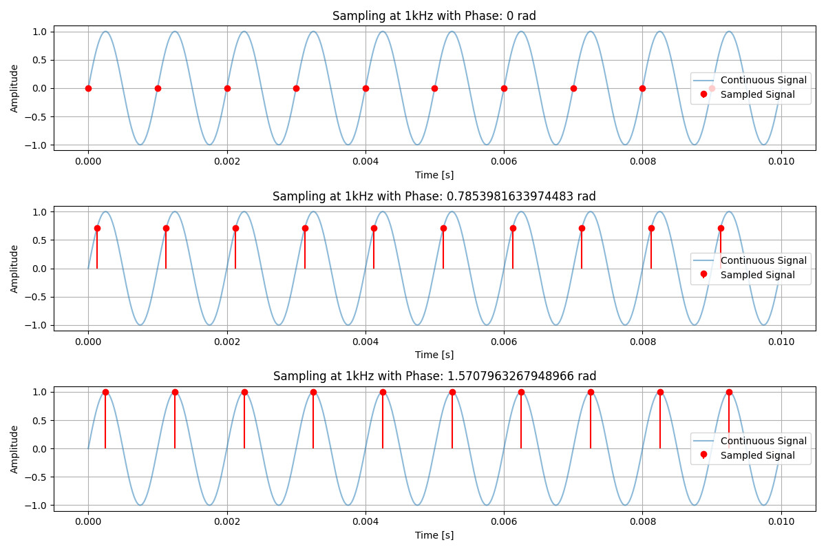
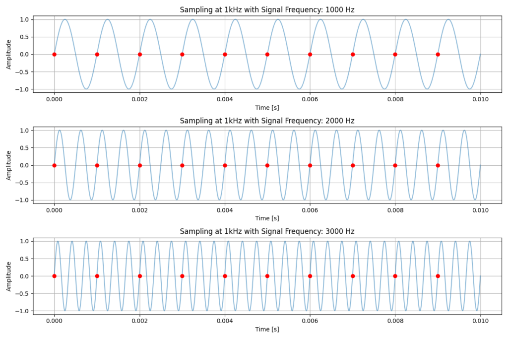
There is no way to use this digitized waveform to work out whether we sampled a 1kHz sine wave or a 2kHz sine wave, since both waves produce the exact same horizontal line. The core idea of Nyquist is that multiple signals can produce the same sampled signal.
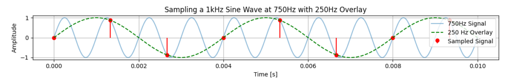
The diagram below also shows the effects of sampling a 750Hz signal with a 1kHz sample frequency. This time, we can connect each of the samples to produce an actual waveform. However, the samples actually give us a 250Hz sinewave rather than a 750Hz sinewave. This occurs due to Aliasing.
Aliasing
Aliasing occurs when different frequencies become indistinguishable after sampling. We saw this in the previous section where the 750Hz sine wave appeared as a 250Hz sine wave. You might think that this just occurs between the Nyquist frequency and the sampling rate but it also occurs above the sampling rate. The diagram below shows us a plot of the original frequency against the reconstructed frequency. We can see that the mapping from original frequencies to the sample sampled frequency is many to one. Therefore, when sampled, each of the frequencies above the Nyquist frequency will incorrectly appear as low frequencies.

In real audio systems, sound sources are not naturally limited to a fixed maximum frequency. If the frequencies above the Nyquist frequency reach the ADC, they will be misrepresented as low frequency signals. To prevent this, anti-aliasing filters can be used to filter out the high frequencies before they reach the ADC. Intuitively, an anti-aliasing filter ensures that the ADC never ‘sees’ frequencies it cannot correctly represent.
Human hearing is usually most sensitive between 20Hz to 20kHz if they haven’t been damaged/aged. For this reason, many music settings use a sampling rate of 44.1kHz. This gives a Nyquist frequency of 22500Hz, which is just above human hearing. Furthermore, anti-aliasing filters will remove any sound above 22.5kHz to ensure it doesn’t get misrepresented as lower notes in the music.
Quantisation and Bit Depth
The sampling rate tells us how many times per second to make a measurement of the air pressure at the microphone. Technically, the electrical signals in the microphone will be continuous representations of the air pressure. The ADC converts the continuous representation into a discrete signal, effectively throwing away information between samples. If we think about this functionally, the sample rate corresponds to the x-axis of the audio function. In reality, the signals are stored as lists but since the sample rate is encoded within the file, the audio card knows how to reconstruct the sound by correctly combining the samples at the right speed.
The digital samples will be stored as numbers, which represent the air pressure (or amplitude of the soundwave). There must be some thought into how many bits to allocate to each individual sample. In other words, the resolution of the y-axis. Similarly to the sample rate, we must also pick a bit depth. In the most simple case, such as older audio recordings from the 80’s and 90’s, a bit depth of 8 bits was set. This means that every sample is stored as a single 8 bit number.
There are 256 possible 8-bit numbers, so there are 256 possible levels for the sample. Many formats use unsigned audio files, which treat level 0 as being full negative amplitude and level 255 as being full positive amplitude. Level 128 therefore reflects the neutral position, in which there is no sound. Below, you can see an example of different bit depths and how they affect the wave. I have shown the difference between 4-bit and 8-bit for a segment of a sine wave.

It is now more common for audio files to be stored as 16-bit for speech or music files. This gives 65,536 possible levels for the amplitude. This allows for higher dynamic range, which is the difference between the loudest and quietest usable signal in the audio samples. It is said to be about 96 dB of dynamic range for 16-bit audio. This difference is hard to notice in many cases and usually presents as noise.
For audio engineers and music producers, it is common to use 24-bit audio, which provides 16.7 million levels and a dynamic range of around 144 dB. Human hearing doesn’t have this much dynamic range however, which means we can’t actually hear the full effects of 24-bit audio, even in a perfect setting.
The reason 24-bit audio is used in a studio setting is to allow additional headroom above a track. In other words, occasional loud sounds are less likely to get clipped by the upper limit of the the available amplitude levels. For a concrete example of this, consider a recording of a jet taking off. Before the jet starts its engines, we might be able to hear workers fuelling the aircraft. Once the engines are enabled, these quieter sounds are quickly drowned out. Finally, upon take off the jet will often exceed more than 120 dB. Although 16-bit audio can theoretically represent this range, recording at such levels risks clipping or forcing the quieter sounds close to the noise floor. In other words, the quieter sounds will need to be quieter in order to fit the upper level of the higher sounds into the reduced number of levels. Therefore, the fuelling sounds will be represented by fewer quantisation levels. Using 24-bit audio allows the recording to be made at a lower overall level, preserving both quiet and loud sounds without clipping. The final playback volume can then be reduced during processing, which is straightforward because the full dynamic range of the original recording has been preserved.
Digital Audio Files
After recording audio with a microphone or editing a song in a studio, it is common to save the file so that it can be accessed later by other editors or consumers. All audio files must contain the following:
- A sequence of PCM samples
- Metadata
- Sample rate
- Bit depth
- number of channels
- encoding format
PCM (Pulse-Code Modulation) is the raw representation of an array of samples ordered in time. For a mono track, from a single microphone, the PCM track will look like [s0, s1, s2, s3, …] for as many samples as there are in the recording. In modern computer audio, it is more common to have stereo audio tracks with individual left and right tracks. You can hear this very clearly through headphones, when a sound moves from left to right. For a stereo PCM, the structure will be [L0, R0, L1, R1, L2, R2, …], which represents left sample, then right sample. Alternating between left and right samples is known as interleaving and is used for efficiency when reading/writing files to storage.
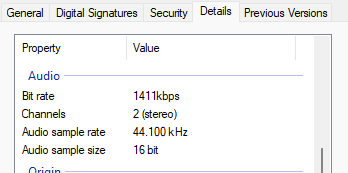
It is common for audio tracks to be compressed in order to reduce the sizes of the files. A common example of this is using the mp3 format, which removes frequencies that are less likely to be heard by human hearing. There will be more on compression in a future tutorial, since it can get quite tricky. Below is an example of audio metadata in the windows properties menu.
Thank you for following along with part 2 of my computer audio tutorial. In part 3, the focus will be on the frequency domain and Fourier analysis. Find part 3 here.
See you in the next one,
Emily